Towards an Audio Angle of Attack Indicator – Part 5: closing the feedback loop

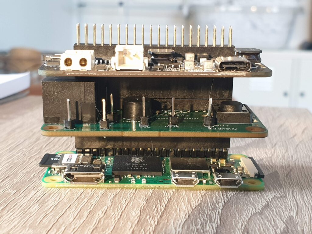
Last time I wrote the challenges I faced with different types of equipment. Because different types of equipment provide me with different supply voltages, different UART signal levels and event different power supply polarities – I decided to introduce modules.
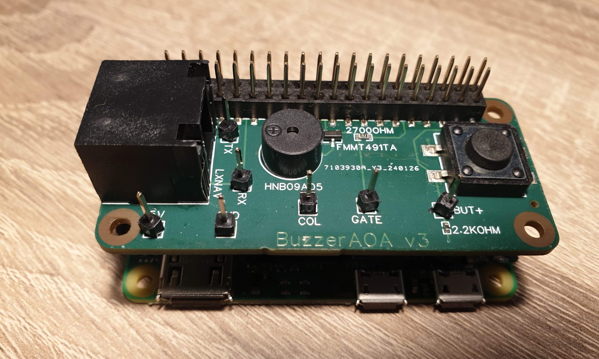
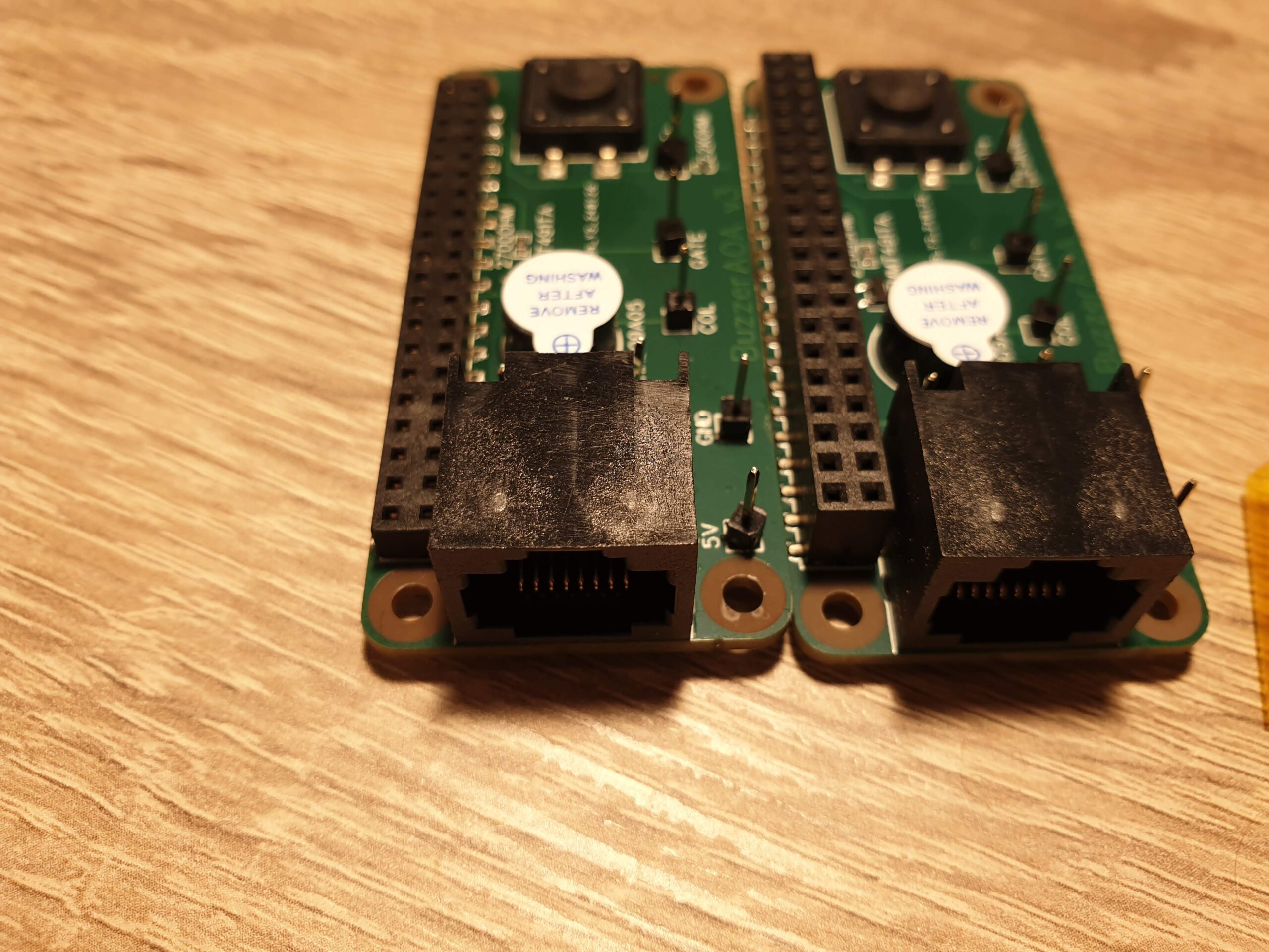
IGC Input Module

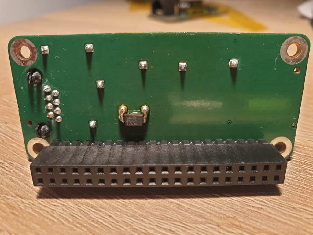
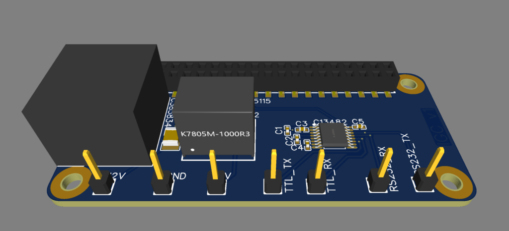
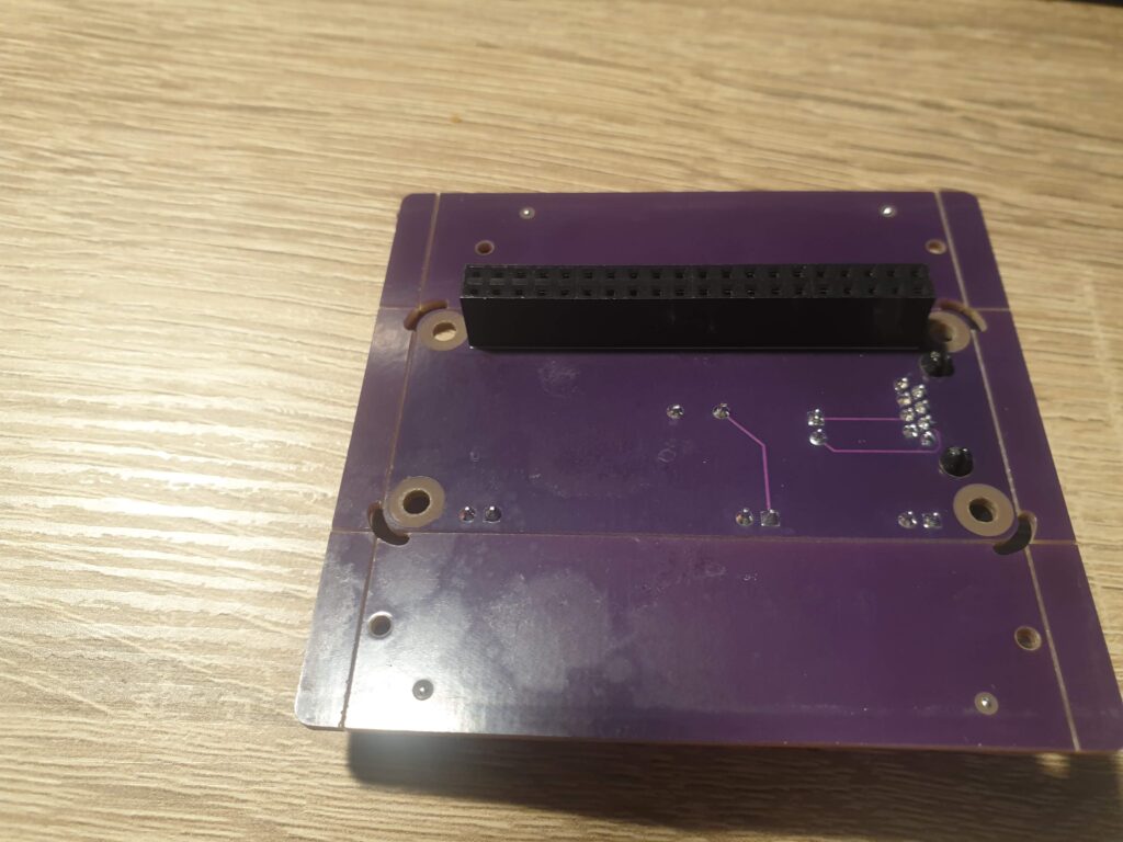
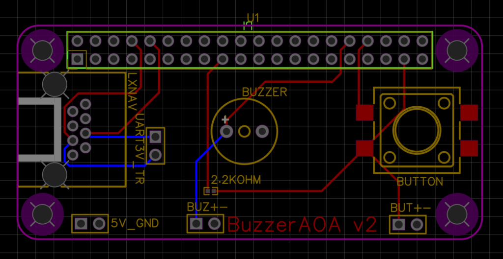
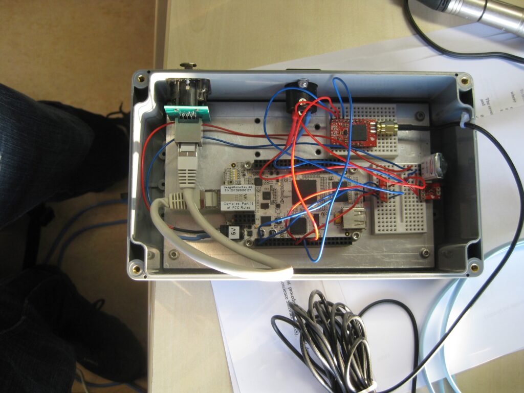
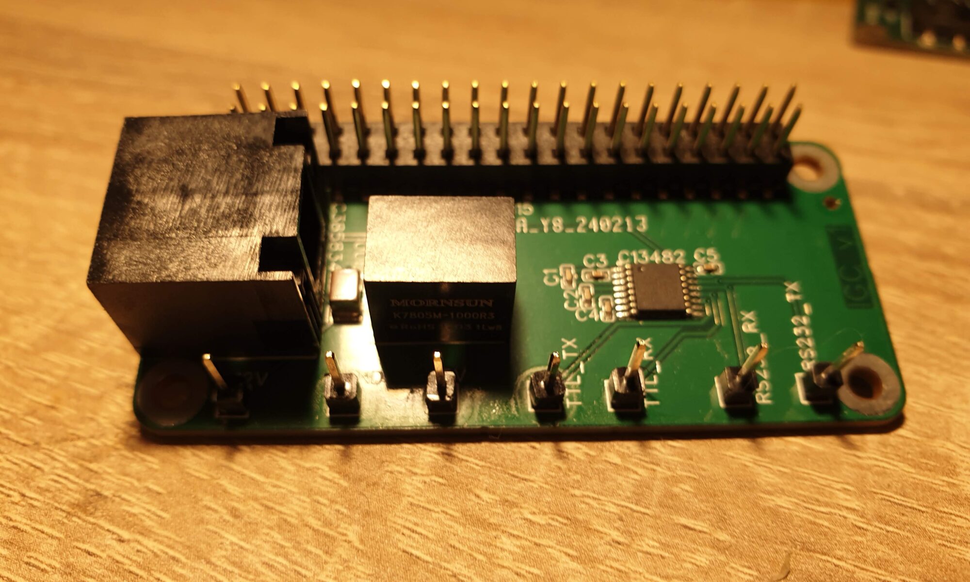
The first module PCBA I ordered was a new Input Module, one that deals with the standard IGC RJ45 pinout. It converts 12 Volts to 5 Volt for the Pi and translates the Pi’s 3.3V UART signal levels to the standard RS232 signal levels of approximately 10 Volts. This was exciting for me, since this was the first time I was doing something more significant than connecting stuff with traces and maybe a resistor here and there. The MAX232 Chip that I used needs a bunch of capacitors to perform its task. The 12 Volt to 5 Volt converter that I used also needs capacitors to work. I now have multiple voltages running over one PCBA: 12 Volt, 5 Volt and 3.3 Volt.

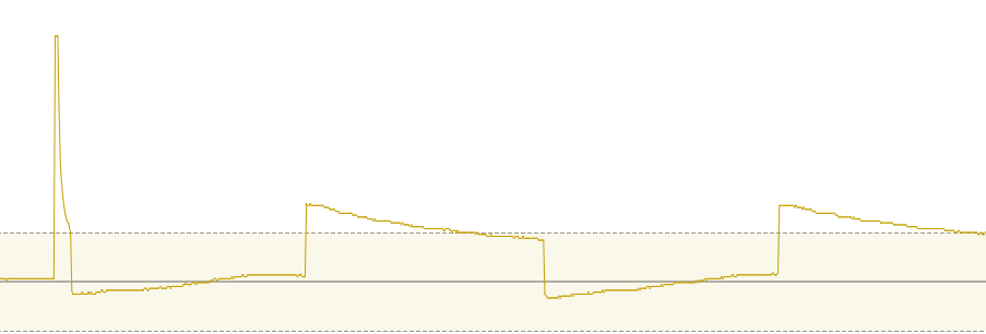
To my delight, everything worked as expected. In order to learn about unit testing for hardware, I wrote a bunch of tests. I can now verify the properties of the DC-DC Converter automatically, using just my Korad KA3005PS programmable power supply and my Hantek 6022BL USB scope. Here is a movie of the test running:

The first automatic test of the DC-DC Converter running

Later on I also verified that the MAX232 setup is working as expected. I have let some friends review my PCBA layout. I’m starting to get more and more confident about creating PCBAs. Even the quality issues I encountered last time, where JLCPCB had placed the wrong part on some of my PCBAs, is now gone. They did have a question about the holes in my PCB being defined two times, so I fixed that.

Now what?

After I verified that this board was working well, progress was slow. There are a lot of things that I can do, but not a lot of things that I have to do. I’m starting to get closer to my initial goal of having hardware that works. So what now?

Last time I mentioned EMC compatibility, fault handling and an enclosure. The enclosure felt useful, but was a bit scary because I have no experience in 3D modelling. EMC is a potentially expensive excercise, but might be important if my enclosure doesn’t block EM radiation. Fault handling feels almost like an academic exercise at this point, and I lack the experience to analyse faults properly.

So perhaps I should just keep doing what I did so far? Improve the PCBAs?

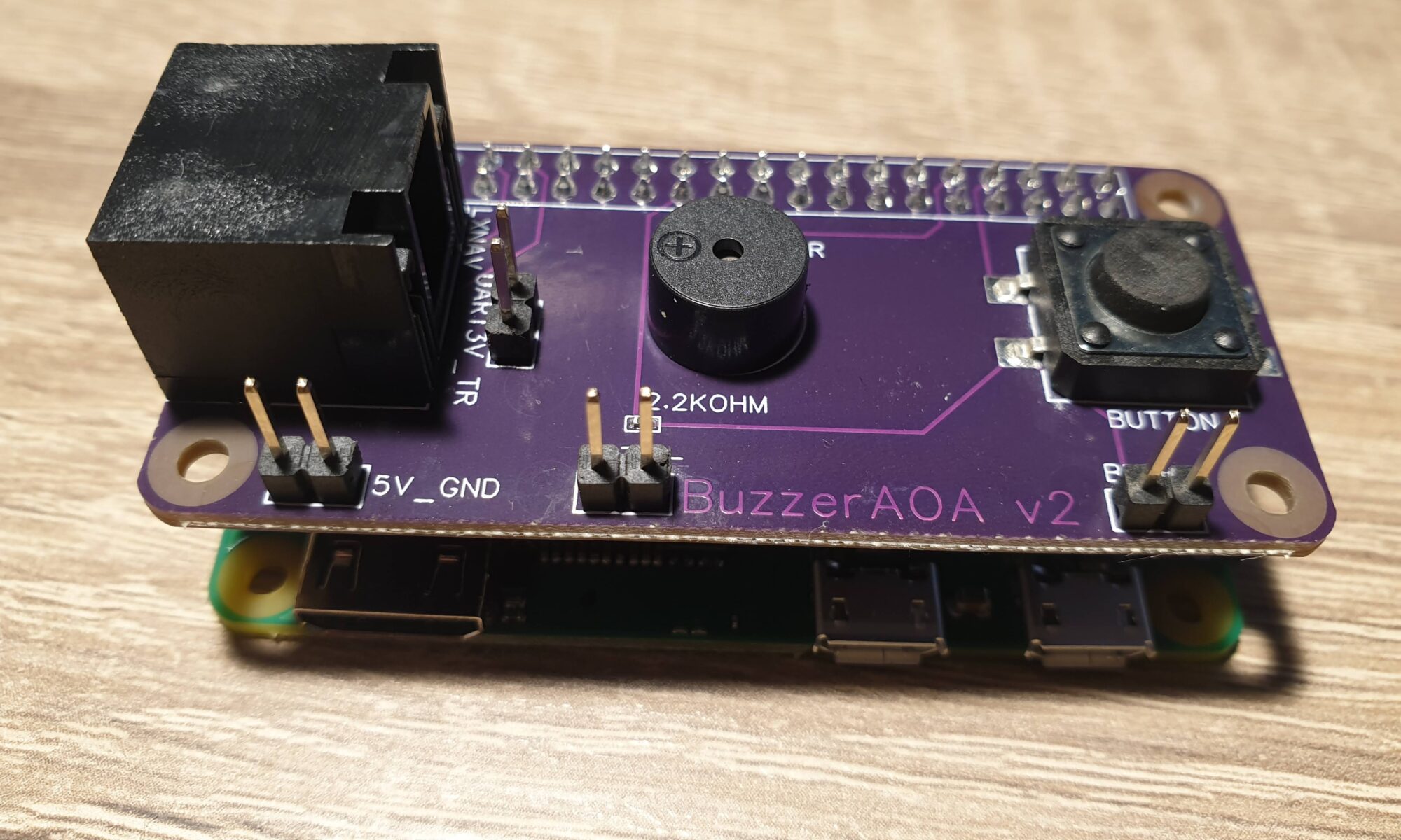
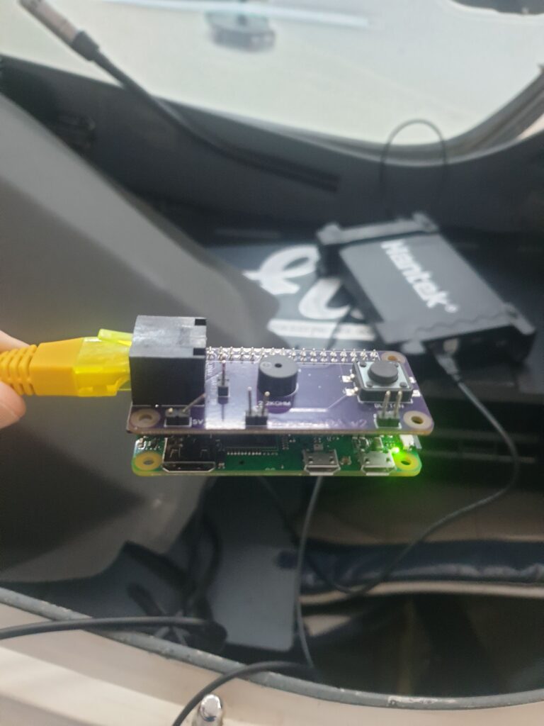
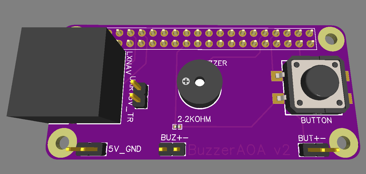
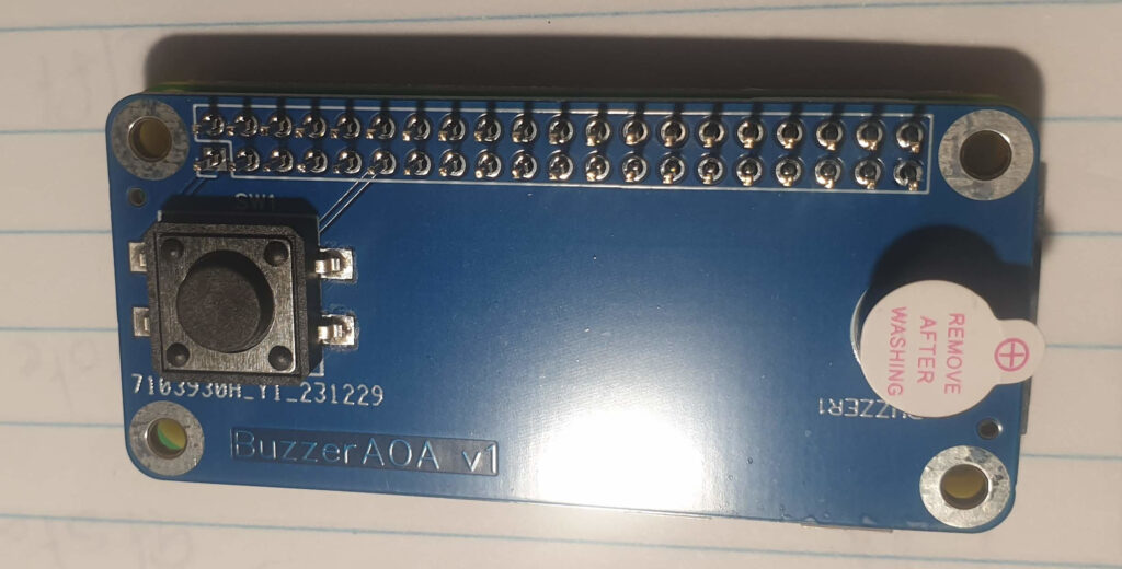
For the Output board, where the buzzer and push-button are currently located, I wondered about placing an RGB led for status indication. It might also be nice to have an accelerometer on the board, which allows me to connect my device with any LX8000/LX9000 device. My gliding club has their entire fleet outfitted with these. An accelerometer might even replace the push-button, if I can use tapping gestures on the device. This makes the device simpler and allows me to make a simpler enclosure. I have not yet gone through with this, because I wanted to test the gesture detection first and see if the 1Hz indicated airspeed that the LX8000/LX9000 devices give out is good enough to give a shot.

I wondered if upgrading the Input board for the LXNAV devices with a current shunt and INA226 current sensor might be a good step forward. This would be a first step towards fault detection and fault tolerance.

Closing the feedback loop

While the above things are nice, they do not bring my system closer to reality. After some thoughts, I decided that the system needs to face reality as quickly and as often as possible. Instead of refining the system over and over based on my idea of what is “better”, I have to face the unforeseen stuff that real-world usage brings.

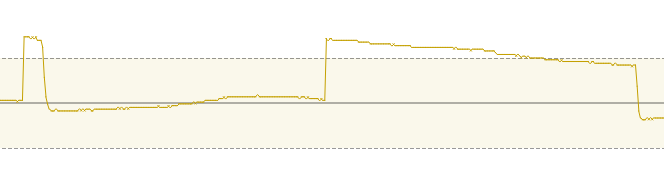
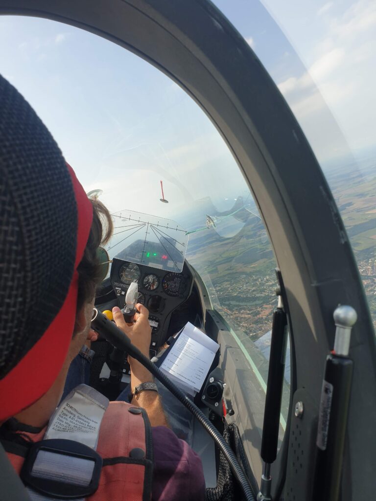
So I decided to step away from PCBA redesign for a bit and focus on other things. I installed Windows 10 and Condor Soaring on an old iMac I had lying around. This allows me to test my system at home. Condor Soaring is capable of sending out the exact values my system needs at 10Hz. This allows me to fly with the system at any time I like.

Testing the system with a simulator brings many interesting lessons. I can no longer start the software myself. What happens when (part of) the software crashes? I’m finding lots of small issues and questions arise.

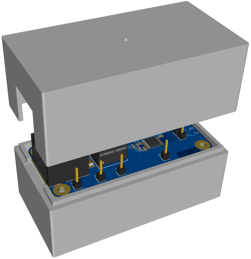
Another thing I did was design and order my first enclosure. EasyEDA Pro has a tool that lets you design an enclosure quite simply. I can then order that enclosure at JLC3DP. It should arrive in about a week from today.

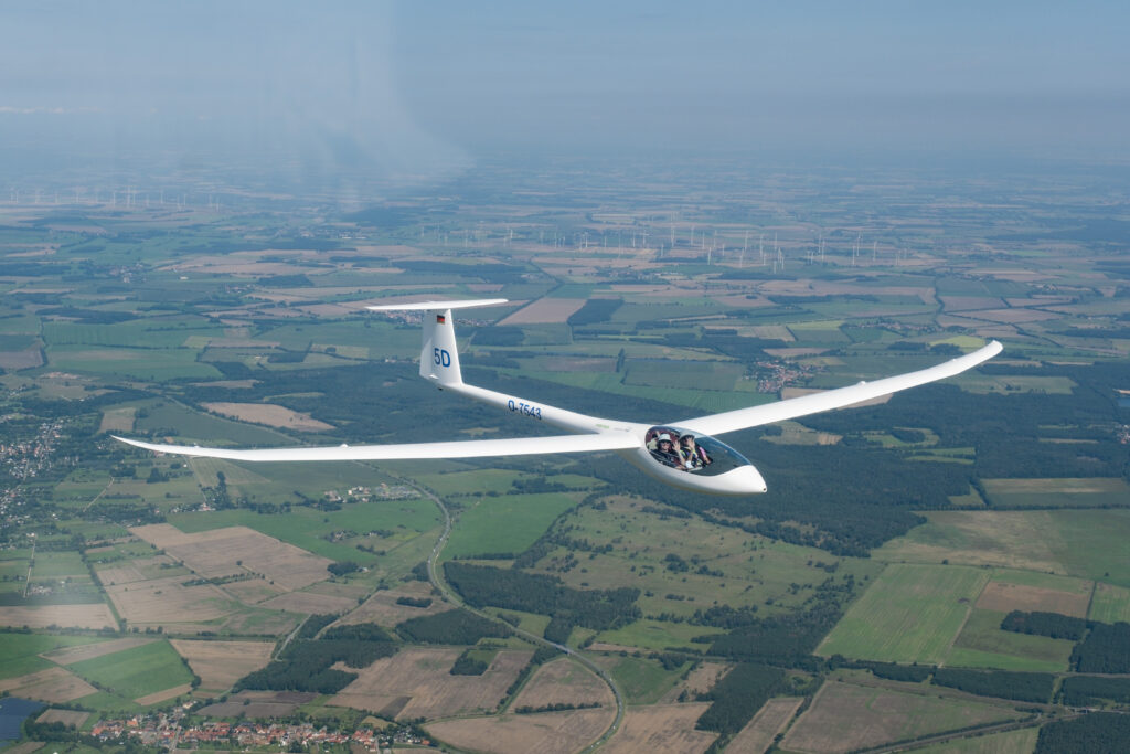
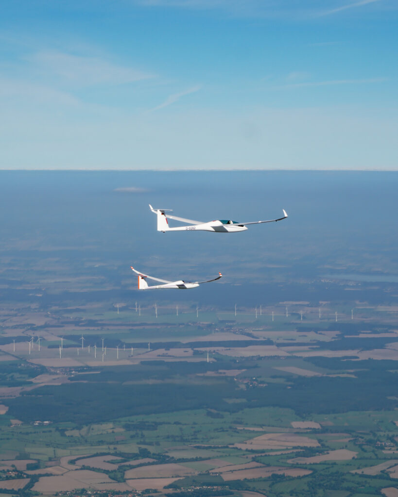
Now that the gliding seasons got started and that I have actually booked my visit to this year’s Idaflieg Sommertreffen in August, I’m eager to start testing my hardware in real life. I can’t wait to use the system and learn more.

Towards an Audio Angle of Attack Indicator – Part 4: Modularity

Last time I wrote about some setbacks. The LXNAV devices that my club owns (LX8000 and LX9000 series), do not support the 10Hz data that I require. This has been the source of a major change in the project: the introduction of modularity.

But before I discuss this major step forward, I should describe iteration 3 of the PCBA.

Changes in iteration 3

There it is. I replaced the expensive female headers at the bottom with female headers at the top. This saves about $50 per order and allows me to stack as much PCBAs on top of each other as I like. But as the picture shows, it was not easy for JLCPCB to select the correct part. Three of the received PCBAs received the tall female headers visible on the right, while two received the correct female headers visible on the left. I off course filed a complaint, which was handled very nicely. The next batch of PCBAs is on it’s way to me as I’m writing this, and I’m curious how they turn out.

Another change is in the buzzer. As mentioned, the previous version had a 3.3V buzzer which was powered by the Raspberry Pi. Because the Pi can only supply a grand total of 51mA (at 3.3V) over all the GPIO pins combined, this solution wasn’t a very good way forward. Iteration 4 contains an NPN-transistor, which I toggle with the Pi’s GPIO pin. The transistor then allows about 200mA to flow directly from the +5V rails to the buzzer. Since the +5V rails is directly connected to the LXNAV device, I have about 1000mA available here. Much better than the 51mA of the GPIO pins!

This version also has the debug pins spaced more evenly over the board, because the lack of spacing was a hazard for shorting two pins in the previous version. The crocodile ground clamp on my scope is simply too large. I did not repeat the GND pin everywhere as well.

Buzzer changes for iteration 4

The spike and oscillation after turning the buzzer off. Yellow band is -5V to +5V

While testing iteration 3, I stumbled upon something that nobody really saw coming. When the transistor cuts the circuit between the Buzzer and GND, huge voltage spikes occur. They were clipped at 25V by my scope, and they appear to be periodic at about 2.2kHz and last about 15 milliseconds. This is suspiciously close to the 3kHz frequency of the buzzer. The electronic experts I consulted suspected it is the membrane of the buzzer which is still vibrating. A colleague was kind enough to solder a diode between the two pins of the buzzer, which should allow any excess current to flow to the +5V line. A quick check with the scope shows this is true: I see no spikes exceeding +7V now, which is great.

A diode soldered across the through-hole pins of the active Buzzer.
The same situation, but now with a diode placed across the buzzer.

Modularity

An example of stacking multiple HATs on top of the Raspberry Pi Zero. The new female headers on top of each HAT allow for an infinite amount of HATs to be stacked.

The last thing to address is the issues I noticed when testing iteration 3 in the workshop of my gliding club: our LXNAV devices don’t send out the data I require to operate!

This has several solutions:

  1. I am now actively looking for private owners who have a glider with an LXNAV S80 or S100. My current hardware should work with those devices, and it provides me with the data.
  2. I am creating a separate version to support LX Navigation devices.
  3. I am considering adding my own accelerometer and seeing if the 1Hz Indicated Airspeed as provided by my club’s gliders is enough to test the system.

Point 2, supporting LX Navigation devices, makes life difficult. Whereas LXNAV provides me directly with 5V and TTL-level UART data, the LX Navigation devices provide me with 12V power and RS232-level UART data. To make matters worse, their pinout is exactly opposite from LXNAV!

After a lot of considering, I decided that this warrants splitting my single PCBA into two separate PCBAs: one for input (UART and Power) and one for output (Button and Buzzer). I can then create two different Input modules – one for LXNAV and one for LX Navigation – and iterate the Output PCBA independently.

The two modules are stacked on top of each other, using the stacking mechanism that I introduced in Iteration 3.

As I’m writing this, the first iteration of the LX Navigation Input Module is on it’s way to me. Since I now have to change the voltage from the 12V battery (providing anywhere between 9V and 18V) to the 5V that the Raspberry Pi requires, I have had to introduce a complete DC-DC Converter module. In order to change between RS232 voltage levels and TTL voltage levels, I have had to include a MAX232-like chip. It was a nice step up from the easier circuits that I had to make before. I’m eager to learn if I got it right. If everything works, this version should also be compatible with other devices that adhere to the IGC standard pinout, like LX Navigation does. That means it should also work with devices like the XCVario.

This is what version 1 of the LX Navigation Input Module should look like. RJ45 connector on the left, DC-DC Converter module in the center, MAX-232 on the right.

Future plans

As the hardware is getting more and more mature, there are some things that I still have not addressed…

I have not performed any ElectroMagnetic Compatibility (EMC) testing. This is something that I should really do before I the system in a glider. The device might otherwise interfere with other on-board electronics. Especially the radio is susceptible to interference in my experience.

I have not made any enclosure for the device yet. An aluminium enclosure might help prevent any EMC issues too. However, I am not yet skilled with 3D modelling. The PCBA design tool I’m using, EasyEDA, does include a 3D modeller for enclosures. Perhaps that is the easiest solution, as JLC also provides 3D printing and CNC services.

There is the aspect of fault detection and fault handling. I have not yet added the LEDs that I talked about last time.

Which brings me to perhaps the most important aspect: getting feedback. Despite all my talk about iteration, I still have to get my hardware airborne. I hope next month I will get the first user feedback.

Towards an Audio Angle of Attack Indicator – Part 3: First tests

Last week iteration 2 of my PCBA arrived in the mail, just a week after ordering. There is a lot of good news, and some disappointments…

First things first. This is what the bottom of the PCBAs look like. There is a 2×20 row of female headers on the bottom, ready to be placed onto the Raspberry Pi’s pin header! For an additional $100, I selected the more elaborate PCBA service with parts placement on both sides from JLCPCB. That means no more soldering for me, and ready-to-use PCBAs right in the mail. This is a bit expensive for my taste, but for the time being it enables me to iterate on my design faster. I will probably move to female SMD headers on the top, which should accomplish the same thing without the hefty pricetag.

The PCBs are now 4 layers thick, with Signals on the outside layers (for easy modification when I make errors) and a 5 Volt and Ground layer in the middle. These planes make save me a lot of individual tracks for 5 Volt and Ground, which makes routing a bit easier. The tracks that I did have to place, I placed such that they are always visible and easy to remove if I make a mistake.

After ordering this iteration, I had some doubts about the buzzer pulling so much current (30 mA) that the Pi couldn’t supply it properly. At first this seemed to be confirmed by my Hantek 6022BL Linux-supported USB-scope, which showed just 2.5 Volts on the pins. Further investigation seems to indicate that it’s actually the scope that’s at fault here. A normal multimeter shows the expected 3.3 Volts. The buzzer also uses less than the 51 mA that the Pi should be able to supply on all of its GPIO pins combined.

It still makes sense to look into powering the buzzer from the 5 Volt plane, using a transistor of some sort to toggle it. After talking to some wise men around me (you know who you are), I decided to re-design the circuit a bit and use an NPN-transistor to toggle the buzzer. I also considered a MOSFET, but that was overkill and introduced the need for voltage divider circuits. I want to keep things as simple as possible, and the NPN-transistor is as simple as I can make it right now.

For the next version I’m thinking about introducing an RGB-LED to communicate the software status to the user. I figure this might be useful when things don’t work as expected. Such a LED uses around 20mA per color, which makes using transistors good practice.

Raspberry Pi Zero booting with power from my PCB for the first time, powered by an LX8080.

Back to this iteration… After the board arrived I quickly checked if things work as expected. The debug pins are very helpful for this, although it would be better to place them further apart. I have no need for connectors, and the ground-clamp on my scope is so big I’m running the risk of creating shorts. Also, it makes no sense to duplicate Ground pins everywhere.

The board works and the Pi boots fine with it. The button now works as intended and the buzzer still works. So then it was time to take the board to my gliding club and test it with real hardware!

The RJ45 pinout seems completely correct! That is a big win for me, since I’m always struggling with pinouts. Matters were not any better this time, as even the numbering of the pins was non-standard in the LXNAV manual. I’m pleased I got it right the first time. The Raspberry Pi Zero boots without a problem using the 5 Volts from the LXNAV, and it can receive the NMEA data from the LXNAV. Progress!

Software

A mild disappointment was finding out that only the S-series variometers from LXNAV support the particular feature I’m using. I assumed from the specification that I had read that any modern device from them would export the needed values (G and IAS at 10Hz). This turned out not to be true. From a first glance at the LX Navigation dataport specification, it should be possible to get the correct data from those kinds of devices. Hopefully the RJ45 pinouts match enough so I can connect to both.

All in all I am quite pleased at how far I have been able to get within a few weeks. I am especially thankful for all the help I have been getting and the encouraging messages I’ve received.

Towards an Audio Angle of Attack Indicator – Part 2: Hello World

Last time, I wrote about the first PCBA being on it’s way. As I’m writing this, the second PCBA is on it’s way towards me. And boy, does it have a lot of improvements…

My very first PCBA!

The first iteration was a “Hello World” of PCBA: it featured just a button and a buzzer. Long story short: the button didn’t work and the buzzer did…sort of.

As soon as the PCBAs arrived, I soldered one onto a 40-pin header and tested it on my least expensive Raspberry Pi: a Zero W. The Pi didn’t even turn on. That’s not good, but it still worked without my PCBA. Although my soldering isn’t that great, it wasn’t the cause for the problems I was seeing: all PCBAs had a short between the button’s terminals.

Button

During design of the PCBA, I decided to tie unused pins from the button to ground. Not such a great move, since I created a short between the 3.3 Volt pin and ground this way. Luckily the Raspberry Pi Zero has some protections and just didn’t power on. No fried hardware yet.

It took me a while to figure this out, but once I did I could easily fix the problem by scratching through one of the lines towards the button. Now the button didn’t work at all, but at least I could test the buzzer.

Another problem with the button was the GPIO pin I had connected it to. Aparently GPIO pin 17 is sometimes used for other things, even though it’s not documented.

Buzzer

The buzzer worked! It made a sound and it was nearly loud enough. A good result for a first try.

What’s next?

First I created an Excel sheet to keep track of which pins I was using and what pins the other Pi HATs I own use. In the future I want to combine my PCBA with perhaps a 12-Volt powerboard and a 5-inch LCD screen.

I then fixed the short-circuit for the button, and started to look at the extra features for the next iteration.

After spending way to long on soldering this PCBA, I decided to see if I could have the manufacturer of the board solder header on it for me. I turned it he can. A few hours of fiddling with EasyEDA later and the 3D view showed a PCBA with female headers attached to the bottom.

The next version should also contain debug points, so I can attach my USB-scope to the board and see what’s happening.

Last, but certainly not least, the board should receive power and data. Lucky for me, this is rather easy. I’m connecting my board to an LXNAV 9070, which delivers 5 Volts of power at a maximum of 1 Ampere. This is precisely what I need and the Pi Zero W can operate well below the maximum of 1 Ampere. The LXNAV also provides a UART interface at 3.3 Volts, which is precisely the voltage that the Raspberry Pi Zero W wants. Since the Raspberry Pi Zero already contains protection against static electricity, there’s no need to build in extra protections at this point. It’s just a matter of routing the correct pins from the RJ45 connector to the correct pins of the Raspberry Pi 40-pin header.

Now that I’m feeding the Raspberry Pi via the RJ45 connector, I’m starting to thing about all the wiring. I remember a former colleague mentioning 4-layer PCBs and I start to investigate a little bit and talk to my electrical engineering colleagues. I decide to create a 4-layer PCBA for the next iteration, just to see if it makes life more easy for me. At JLCPCB, who I use to create my PCBAs, it makes no difference at all if I use 2 or 4 layers… so let’s try it!

Both the UART and the 5 Volt circuits get their own set of pins for attaching a scope, and I order the next version of the PCBA. Since I decided to place parts at both the top (button, buzzer, RJ45 connector) and the bottom (female headers to save me some soldering), I now have to move to a more expensive price category…which is about $100 extra compared to the previous iteration. That’s definitely something I’m going to look at for version 3.

After ordering, I’m again faced with the long wait for these PCBAs to be made. Although the week it takes JLCPCB to manufacture and send the PCBAs is quite quick by modern standards, I’m so used to feedback loops measured in seconds or maybe minutes that this feels like going back in time. Despite feedback being somewhat slower than I’m used to, I’m quite excited about this small project. I’m learning new things every time I’m working on this project, and people all around me are very willing to teach me. No amount of studying beats experience…

Towards an Audio Angle of Attack indicator – Part 1: Inspiration and simulation.

We all know that Angle of Attack (AOA) is the measure of our approach to stalling. However, in general aviation we don’t measure or display it. I’ve always thought that it’s a shame we don’t; in military aviation the use of AOA is ubiquitous, reducing pilot workload. Most military aircraft even show the AOA in their Heads-Up Display (HUD), both as a value and in a projected velocity vector. In my experience flying military simulators, this makes landing quite simple.

Since we fly large portions of our flight at a high AOA, I thought it would be valuable to have the pilot know their AOA. We don’t have fancy HUDs, so we would need to convey the AOA information in another way to the pilot. Both DG and the Akafliegs have used “Seitenfaden” – strings at the side of the canopy – with good results.

A flight in a SF-34 with the forward instrument panel covered. Source: YouTube./AKAFLIEG Köln

These side-strings work well, but they have to be looked at and interpreted by the pilot. Interpretation of visuals happens in a relatively recent part of the human brain, and requires more effort than processing sound or tactile information. I’ve experienced this when I navigated through a city using just a tactile car seat myself. So I started looking for ways to convey the AOA – a pretty vital piece of information – by sound or touch. Then I stumbled upon an existing audio AOA indication, which was present in the F4 Phantom jet.

A video game demonstrates how roughly the F4 Phantom’s AOA warning worked. Source: YouTube/CAFubar

Idaflieg

After last year’s Idaflieg Sommertreffen, I decided that for 2024 I wanted to test a more intuitive version of an AOA system. Idaflieg’s Zacher experiments, where students take their first steps as test pilots, provide the ideal environment to test such an experimental system. The goal is to provide the pilots with a small electronic device that can easily be plugged into the existing instrumentation, does not require too much workload to operate and will always give an audio indication of your AOA.

Design

It is probably easiest to approximate the AOA by the Lift force, as we can calculate it from the Indicated Airspeed (IAS) and the Load factor (G’s). After indicating what the system should consider as the maximum AOA, it can estimate the AOA in most situations.

Simulation with Condor Soaring

The first step was to write simply try something and simulate it. So I did: I wrote a Linux program which receives Condor Soaring’s UDP information 10 times per second and estimates the AOA. It them generates 100ms worth of sound to indicate the AOA to the pilot.

When I tested this with Condor Soaring, the result was very pleasing. It became pretty effortless to fly steep turns with a glider, right on the edge of stalling. During loops you also get valuable feedback for flying your figures well. During landing it allows you to direct your focus to the outside world and not scan your airspeed indicator for things like wind-shear.

Simulation of the AOA indication on an aerobatic flight from 2016, in a Pilatus B4AF.
Turn your sound on. The “clicks” indicate the AOA: the closer to MaxAOA, the faster the clicks.

Overall, flying in the simulator felt more relaxing. Funnily enough, this was also the major problem that instructors mentioned when I asked them if they would consider such a system for their students. With increased automation and assistance comes an increased risk of automation complacency.

Overall I’m pleased with the results of the simulation. The next step will be creating a small device that the pilots can actually bring during the next Idaflieg Sommertreffen. This requires me to learn something new: designing Printed Circuit Board Assemblies (PCBAs). As I’m writing this, the first iteration of a PCBA is on its way to me…

The Akaflieg Braunschweig SB-14 – an exercise in minimalism

As a result of my education in embedded systems programming, I’ve come to respect minimalism. Perfection – for me – is found when there is nothing left to subtract.

Shortly after my arrival in Stendal, I made my way to the enormous glider hangar. I had never seen glider prototypes and I was keen to have a look at what the Akafliegs brought to Stendal this year. There I met the Akaflieg Berlin B-12, the FTAG Esslingen Apis Jet, but one glider stood out for me personally… the Akaflieg Braunschweig SB-14.

The SB-14 has to be one of the most slender composite sailplanes that has been produced so far! An exercise in minimalism. Function dictates form. I love it! During my visit the SB-14 regularly flew test flights, and I spoke to some people who designed parts of this sleek machine. So I just had to know more, and started to talk to Lars Samake, project leader for the current certification efforts.

The SB-14 in flight, Lars at the controls. Photo by Simeon Schmauß

In contrast to some other Akaflieg designs, the SB-14 was not designed to test a new concept. Instead the goal was to minimize the surface of the fuselage compared to other gliders. To further reduce drag a special wing profile was designed, where the transition from laminar to turbulent flow happens very late. The airflow is forced from laminar to turbulent using boundary layer blowout holes, similar to what some other gliders (DG-300, ASG-29 and others) use.

The SB-14 had it’s maiden flight already in 2003, and has flown under a Permit to Fly ever since. As with most Akaflieg projects, the goal is to create something which passes certification, so the intention has always been to finish certification. Certification to JAR-22 was started in the past, but never finished.

The flight tests during the Sommertreffen of 2023

In the past few years, the “high risk” tests for JAR-22 have already been performed. These include tests like extending the airbrakes at 1.05 times the intended Vne.

This year it was time for calibration of the airspeed indicator, checking stalling behavior, checking the air brake effectiveness, control forces, stability… you name it. The goal was to perform two certification flights per day.

Two flights per day doesn’t sound like that much, but each flight should be thoroughly prepared the evening before the flight. During the flight everything is filmed, so an additional one to two hours of evaluation takes place after the flight. During the first weeks of the Sommertreffen, Lars did all these tasks himself, but he was happy to leave the flying to another pilot once a more aft center of gravity was required. During the whole process, Lars was supported by the members of Akaflieg Braunschweig and pilot with extensive flight test experience, and the LBA is also present during the Sommertreffen.

Evaluation of the airflow over the fuselage using tufts. Source: Youtube/AkafliegBraunschweig

What’s next?

So what’s left for certification? The same tests that were performed this year should be performed with water ballast, in order to test the glider at the maximum take-off weight. These include tests evaluating stall speed, stall characteristics, general flying characteristics and take-off/landing behavior of the glider.

I can’t wait to see this beautiful glider back in the air next year. Hopefully for the last time with a Permit to Fly…

Flirting with wireless networking

Any sufficiently advanced technology is indistinguishable from magic.
– Arthur C. Clarke

Planting seeds

Wireless networking has always felt like magic to me. Two computers talking to each other with no shared base just feels special. Thus, it was no surprise that I took several courses on wireless networking in my Computer Science Master’s degree. It just made sense.

I wasn’t disappointed with the basic courses, covering systems like WiFi, 3G and hearing commercial pitches for 4G/LTE and WiMax. But my imagination was really sparked when I did the course on wireless mesh networking. The vision of large amounts of systems talking to each other without depending on any infrastructure, this felt like science fiction to me.

During the course we studied many existing systems – such as AODV, ODMRP and SMAC – and were challenged to critique them and propose improvements. This has been one of the best courses I have followed during my Master’s. I was simply mesmerized. Another course focused on using these wireless networks to autonomously monitor environments: wireless sensor networks.

During this time I took regular walks on my university’s campus and I would often lie for hours in the grass, looking at the clouds pass. Then, one day, a glider from the nearby airfield came circling above my head at low altitude. Another one joined.

A thought involuntarily cross my mind: “What if we could map the structure of thermals in real time with a wireless sensor network?”. And thus, the subject for my Master’s thesis was born…

Master’s Thesis and a paper

I was able to convince the Pervasive Systems research group to let my do my Master’s thesis on the concept of “Wireless Mesh Networking for Gliders”. During my 9 months of research I selected the X-Bee Pro 868 transceivers has my hardware of choice. With a range of 40 kilometers, I expected they would be a good choice despite the low bandwidth. And since FLARM had already received exemption from the ground-only usage for the 868MHz band, I figured I could use them too. I used many IGC files to simulate what good days and bad days would look like in terms of connectivity. The potential is there, but routing data over a Wireless Mesh Network was harder than I could handle, especially since end-to-end connectivity between two gliders was rare. I designed a protocol based on epidemic routing, where nodes forward data based on probability rather than a strategy.

A potential wireless mesh network that could be formed during the Dutch National Championships.

Meeting my heroes at OSTIV

Although my solution worked “okay” – I could deliver 80% of all data – my paper was accepted at the 2010 OSTIV conference in Szeged, Hungary. And since my university’s policy was to pay the expenses for attending any conference that accepted your paper, I got myself a free trip towards the World Gliding Championships in Szeged! I met many of the famous constructors: Loek Boermans, Mark Maughmer, Gerhard Waibel and Johan Bosman. They were all extremely welcoming and a lot of fun to hang out with! I presented my paper and received a prize for best (only) student submission. I had a blast.

Right after the conference I started working and had very little time to work on my project. I realized that there is an inherent chicken-egg problem in wireless mesh networking: you need others to pass your data along, and very few people are willing to be the first buying such a system. Also, the problems in efficiently carrying data from glider to glider persisted.

But there was also good news: OGN launched! Although coverage at the time was not great, it was a start. There was also live tracking by SkyLines, which worked over 3G. At first I thought both systems were too limited in their coverage. From experiments during several tows to 1200 meters during aerobatic courses, I learnt that coverage stopped at around 600 meters above ground. This improved, but I didn’t know it….

A revelation

…until I decided to perform another experiment. Since I had been running a backup for the SkyLines project, I had access to their database. And this database included the tracking information. I could see that 97% of all position reports arrived within 1 second! That meant that in 97% there was very likely a connection between the glider and the internet! This included flatland such as The Netherlands and the Alps. I figured my assumptions about connectivity were false, that it didn’t make any sense to continue working on the hard problems of wireless mesh networking and decided to just use 4G. I bought a 4G modem and started testing with it, and connectivity was indeed great.

Although this sadly removed any need for wireless mesh networking for gliders, it did free me to pursue the next step: figuring out what to measure and share it. More on that in a separate post…

Forschen, Bauen, Fliegen with Idaflieg in Stendal

Ever since I started my studies in Computer Science, I started to fiddle with electronics in gliders. I enjoy this very much, except for one small part: explaining this to other glider pilots. Most glider pilots I meet roll their eyes when I passionately talk about electronics in gliders, and mumble something like “But why?”.

Getting a bit tired of trying answer that question, I started to look online for like-minded people. And so around 2010 I found out about Idaflieg, the umbrella organisation of the German Academic flight clubs (Akafliegs), existed. Following their motto “Forschen – Bauen – Fliegen” (Researching – Building – Flying), they not only teach you to fly. They also perform research and build their own prototypes, quite successfully. It’s no surprise that most well-known glider manufacturers employ former Akaflieg members. Their prototypes also inspire these manufacturers. Perhaps the most recent example of this is the Mü31, whos influence can be seen on the high wing position of the Jonkers JS3.

Idaflieg collaborates with the German Aerospace Laboratory (DLR), which provides their beautiful Discus 2c DLR with instrumentation and personnel during the yearly summer meeting, the Sommertreffen. During 3 weeks, Idaflieg and DLR collaborate at Stendal airport to measure the performance and flight characteristics of gliders, perform their own experiments and certify their prototypes.

Visiting the Sommertreffen was on my wish list for about 10 years now, but I somehow never got around to it. Around new year of 2023 it started to hit me: I have to visit this event! No more postponing, this is the year. And so I drove via my club’s summer camp in Wilsche to Stendal.

Aftermovie Idaflieg Sommertreffen 2022 – Idaflieg e.V. / Lars Samake

The first night, I start to talk with Carlos of Akaflieg Stuttgart. He asks me who I am and why I am visiting. I expect the “why” question, but it doesn’t come. Carlos starts to tell me about his club’s project: fs36 – the first certified glider with fly-by-wire technology. Carlos tells me it’s pretty difficult, because none of the CS-22 regulations are written with fly-by-wire technology in mind. Therefore it’s up to Carlos and his club to prove their system is safe enough to be certified.

Zachering

The next day I receive my instruction in Zachering, a systematic method of evaluating the handling of gliders named after it’s original author: Hans Zacher. By flying prescribed maneuvers and using just a stopwatch, tape measure and protractor, one can evaluate many aspects of a glider’s handling. Carlos asks me to join him in the evaluation of a brand new DG-1001 Neo, an offer I can’t refuse since I regularly fly aerobatics on the DG-1000S with 18-meter tips. My club has the “old” 20 meter tips too, and I don’t like them.

We tow to 1800 meters and retract the electric landing gear. First we look at the stalling behavior of the glider. We stall the glider straight and level, with 10 degrees of side-slip and in a steady 30 degrees turn. I notice that the DG has become more docile with these new tips, especially compared to the old tips I don’t like. There are lots of warnings before the glider stalls, and with 10 degrees of side-slip there is a tendency to enter a stable turn with some shaking and mild rocking.

Carlos flies a 30 degrees turn.

Next up is the behavior related to adverse yaw. We roll a few times without using any rudder input and note for the time needed to reach 30 degrees of bank. We also estimate how much yaw is introduced as a side-effect of rolling. We also perform the inverse maneuver; from a stable 30 degrees turn we roll back to wings level using just the rudder. Finally we measure the time to perform a 45 degrees left to 45 degrees right turn. The DG seems more agile in 20 meters than I’m used to. I’m starting to be impressed with these new tips!

We enter a thermal together with the Akaflieg Darmstadt D-43, a side-by-side two-seater. The D-43 looks sleek when it flies over the iconic church of Stendal. Again I’m surprised by the low control forces of the DG.

The Akaflieg Darmstadt D-43. Photo by Simeon Schmauß

The next day we continue our program. Next up are maneuvers to determine the stability of the aircraft, which requires still air. We begin with the dynamic stability in the pitch axis. After we release the tow, the DG is trimmed to 115kph and slowly decelerated to 100kph. After the stick is released, the aircraft enters a phugoid. The DG dives down and lifts the nose up at 130kph. I start my stopwatch and Carlos writes down 130kph. The DG slows down and lowers the nose, and Carlos writes down the minimum speed. The DG picks up speed again, accelerates to about 130kph and starts to lift the nose again. I time 27 seconds and Carlos writes down the airspeed. We continue this 6 times, and conclude that since the speeds at the top and bottom of the oscillation do not diverge the DG is currently dynamically stable in pitch.

Finally we look at the forces needed to fly different airspeeds. While having the aircraft carefully trimmed at 115kph, we fly different speeds and note down how much force should be exerted to steadily maintain that speed. We also look at the required stick deflections.

After about 40 minutes we’re done with the program and land. Next up is an evaluation of the cockpit and checking our results with an experienced Zacher instructor. If our results are good enough, they will be entered into a central database. Using this database one can then compare our results of the DG with the results from other gliders.

Performance measurement

After evaluating the DG with Carlos, I help with preparing a Glasflügel 304 for performance measurements. This particular 304 has been measured already once in 1981, but using a different reference aircraft. Measuring it again can reveal differences between the two reference aircraft and their setups.

A complete day is spent cleaning, polishing, documenting (every little scratch and bubble in the gel coat is carefully described), instrumenting and finally weighing the glider. At the end of the day the 304 has been fitted with a very precise GPS received and a WiFi connection for communication with the reference plane. The plane is weighed with the pilot on board and parked in the front of the hangar.

The next day my alarm clock goes of at 05:20AM. This is when the decision is made: is the weather favorable for a turbulence-free performance measurement? The weather looks good, and at 05:45AM the Discus 2c DLR, the Glasflügel 304 and two tow planes are transported to the runway. Everything is set up on the runway of Stendal and the tow planes tow the gliders to 3000 meters. To prevent the pilots from getting bored, quality German music is played over the radio. The gliders are towed into formation and release. For each data point, they fly the same airspeed for a few minutes in formation. Meanwhile the measurement system records their vertical speed precisely at 10 times per second.

After about an hour the gliders fly over the airfield in formation and land. A DLR employee starts to extract the data from the Discus 2c DLR. He shows me a plot with the measurement from 1981 and today’s measurement. The data looks good: as expected there is a slight degradation in performance compared to 1981.

After a week I drive home extremely inspired. I’ve learned a lot, I’ve seen lots of awesome prototypes (more on those in separate posts) and I’ve even been able to help a little bit. I can’t wait for next year…

My first baby steps in avionics and flight testing

Moving map

I started both gliding and my studies in Computer Science in 2003. A few years later, in 2006, things started to itch. I looked at the state of glide computers at that time, and wondered: “Why are these things so expensive? I bet I can do better!”. So, as part of a project on embedded systems, I wrote a small moving map display for an iPaq 5550. The software was very simple: it would connect over Bluetooth to a GPS and display a trace on Geocover2000 tiles that I downloaded from NASA’s WorldWind server. The color of the trace showed a GPS vario value measured at that location.

This system was easy to use, and because I owned no glider at the time, I took it along for some flights in my club’s Ka8.

First variometer

All this was very nice, but I quickly realized that in order to do anything remotely useful, I would need to measure a properly compensated variometer value. And, having measured this compensated variometer value, it should be shown in a friendly manner. I owned a Pilatus B4, so I could finally integrate some electronics.

I decided to start with the variometer gauge first, and I was able to convince Mike Borgelt to share with me the protocol for steering the second-seat version of his variometers. I bought a Beaglebone, a BMP085 barometric pressure sensor, a USB-to-RS485 dongle for the Borgelt gauge and a casing and started experimenting.

The first measurement box, with a Beaglebone, GPS receiver and a BMP085 barometric pressure sensor.

The first test revealed something important: all these electronics are interfering with my radio! Every time I turned on my newly made electronics box, the radio would constantly start receiving noise. No amount of squelch could prevent this.

I told one of my colleagues with an electronics degree, and he suggested I put aluminium tape on the inside of my electronics box. Scratching the tape made the different layer contact each other and would shield the outside world against EMC from the Beaglebone and the switching 12-to-5 Volt converter I used. This made matters much better, but interference would still be present whenever I ran cables next to my glider’s power supply cabling. A piece of ferrite finally fixed things enough so I could start testing my new uncompensated variometer gauge. To the airfield!

The first test flight of my cockpit-pressure variometer. The bottom-center gauge is my own variometer.

This variometer used a simple Kalman filter to reduce the noise in the vario signal. Using some known information about the Pilatus B4 like its stall-speed, I could assign confidence numbers to the noisy readings I was getting from the BMP085. This allowed my Kalman filter to reduce the noise from my measurements, by looking at what’s physically likely to happen.

Measuring polar curves

During the same period I had followed a course on Modern Design of Experiments (MDOE) at work. The basic premise of this course is that – given a clear objective, a physical model of the phenomenon to be measured and a required accuracy – one can derive a mathematical model (response surface) of a system using just a few strategically chosen measurements. This contrasts the more traditional method of taking a lot of data and thinking about the mathematical model afterwards. In wind tunnels it saves a lot of measurement time, so it might reduce the number of datapoints I need to measure to get a plausible polar curve for the B4 too.

I had already obtained a polar curve of the Pilatus B4 from Idaflieg, so I had a pretty good idea what my results would look like. With this information, I could pick the few measurement points that I should measure. Since most software uses a formula of the form a*x2 + b*x + c, I opted to use that as well. That meant I would want to measure at the extremes, the points with most leverage, to determine the linear part of this function optimally and measure right in the middle to determine the quadratic part optimally.

I towed to 2 kilometers and flew timed descents on MacCready 0 speed, MacCready 5 speed and in the middle. In order to estimate the average wind direction and wind speed, I flew a few circles with constant speed and heading in between each pair of measurement points. The drift in these circles would give me an estimate of the horizontal wind.

The results looked pretty okay. As expected, my Pilatus B4 performed a little bit worse than the one measured at Idaflieg. That was not a surprise to me: I had some scratches on the leading edge of my wings, and the fairing at the wing-fuselage intersection was deformed from assembly mishaps. Taping was no longer possible. I also flew the glider mainly for aerobatics, so it didn’t receive the TLC one would give to a high-performance cross-country glider.

Although I realized that I still had a lot to learn and technical challenges to overcome, being able to derive a plausible polar curve using just a noisy barometric pressure sensor inside my cockpit was encouraging. In the meantime I had learned about statistics and implemented my first Kalman filter! I had evaluated the filter in terms of resonance and response time, and it had worked in practice! I was hooked, avionics became my poison.